Quantum Monte Carlo Meets the Balance Sheet
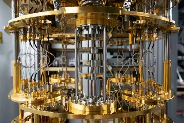
A dilution refrigerator used to test quantum processor prototypes.
Credit: Agnese Abrusci
Making Monte Carlo faster by calling a QPU inside a normal finance workflow
Banks and insurers live on Monte Carlo—running thousands or millions of random scenarios to price options, test hedges or estimate value-at-risk. The method is accurate but slow because error drops only as the square root of the number of paths. The quantum twist is quantum amplitude estimation (QAE), which estimates averages with quadratically fewer samples in theory. In practice you don’t replace your stack with a quantum box; you add a quantum processing unit (QPU) as a step inside the job and keep everything else (data prep, risk logic, reporting) on CPUs/GPUs. That hybrid pattern is what recent research and cloud runtimes now support.
What “quantum Monte Carlo” actually means in finance
Here it means: keep your classical payoff logic, but have a QPU sample the distribution more efficiently via QAE, then hand the estimate back to the classical code that calculates prices or risk metrics. IBM’s option-pricing work laid out the blueprint—encoding payoffs into circuits so QAE can estimate their expectation value—showing how vanilla, multi-asset and barrier options fit this mould. The promise isn’t magic; it’s better error–time trade-offs for the same finance maths.
Two terms worth decoding as they appear. Transpilation is the compiler step that rewrites your circuit to fit a specific device’s layout and native gates, keeping depth—and therefore error—down. Primitives (such as Sampler and Estimator) are vendor APIs that wrap transpilation and execution so you can call a QPU without micromanaging hardware details; they make jobs auditable and repeatable as devices evolve.
Where the speed-up comes from—and the catch
Classical Monte Carlo reduces error like 1/√N over N paths. QAE, in the ideal setting, reduces error like 1/N—hence the “quadratic speed-up.” That’s the theory; the catch is noise. Today’s devices introduce errors, so practical variants (for example, maximum-likelihood or iterative amplitude estimation) trade some of the asymptotic gain for robustness on real hardware. Good articles now compare these families and when to use which. The headline remains: if you can load the distribution and payoff efficiently, QAE can reach a given accuracy with far fewer circuit evaluations than classical Monte Carlo needs.
How this plugs into an actual job
Cloud runtimes package the hybrid loop so teams don’t stitch it together by hand. Amazon Braket Hybrid Jobs spins up your classical Python code, gives it priority access to the chosen QPU during the run, and tears the environment down when finished—keeping logs, configs and metrics in one place. Microsoft’s Azure Quantum Elements shows the same orchestration mindset on the chemistry side—AI and high-performance computing (HPC) wrapped around optional quantum calls—which is a helpful template for governed finance pipelines too. The aim is boring reliability: versioned circuits, explicit runtime settings, and results that auditors can reproduce.
What you use it for first
Option pricing and XVA. Encode the payoff so QAE estimates its expectation under your risk-neutral model, then let your classical code handle discounting and aggregations. IBM’s methodology paper shows how to do this for single-asset and path-dependent payoffs. The win is fewer effective “shots” for a target error bar, which matters when overnight windows are tight.
Risk measures (VaR/CVaR). Use quantum circuits to sample tail behaviour more efficiently, then pass candidate estimates into your existing VaR/CVaR calculators. Recent preprints demonstrate end-to-end scenarios—equity, rates and credit—by building stochastic models as circuits and joining them to QAE. The design is still research-grade, but it illustrates the full pipeline.
Portfolio sub-steps. Some allocation problems embed expensive sampling (for example, scenario picking or stress mixes). A QPU can propose estimates more quickly, while the classical optimiser enforces constraints and produces the final weights. This is “quantum for the sampling, classical for the rules.”
What changes in the developer experience
On the quantum side you’ll define: (1) state preparation (how inputs, such as a normal or log-normal factor, are loaded into a circuit), (2) the payoff encoding (so the circuit’s success probability reflects the quantity you want), and (3) the estimation routine (QAE flavour and depth). On the classical side you’ll keep the model calibration, cash-flow logic and risk reports. Vendor toolkits help with the quantum pieces: primitives hide device specifics, while documentation now exposes tunable options (for example, resilience levels or dynamical decoupling) that act like “noise-cancelling” for circuits.
Limits to be honest about (and how teams work around them)
Noise and size. Today’s QPUs are still small and imperfect. That’s why you’ll see robust QAE variants and error-mitigation turned on by default, with progress toward error-corrected logical qubits—the building blocks that improve as you scale—tracked in peer-reviewed milestones. You don’t need perfection to experiment; you just need transparent settings and classical cross-checks.
State-prep costs. If loading the distribution is expensive, the end-to-end advantage can vanish. Current papers either build the stochastic model directly as a circuit or reuse structure (for example, low-rank factor models) to keep circuits shallow; that’s where most engineering effort goes today.
Benchmarking fairly. Compare like with like: target error (in basis points), wall-clock including queue time, and total cost—including simulator baselines. Many vendor guides and talks now emphasise this governance so results don’t drift with compiler updates.
How to make it purchasable (a buyer’s checklist)
Show the workflow. Diagram the classical parts, the QPU call, and the hand-off back to pricing or risk code. Braket’s job wrapper is a good example of how to keep artefacts and logs in one place.
Explain the trade-offs in sentence-length English. “We use a QPU to estimate an average with fewer samples; we keep the model and constraints classical; we validate against a CPU baseline on control instances.” Back this with links to the option-pricing method and QAE theory.
Package like any accelerator. Offer standard SDKs, SLAs for job queues, and clear change notes when back-ends or compilers update, so audits pass without drama. Vendor primitives exist precisely to stabilise this interface as hardware evolves.
Beyond Monte Carlo: other quantum paths
There are other quantum routes besides Monte Carlo. For decision problems you can cast as optimisation—such as portfolio construction or rebalancing under hard constraints—teams are testing variational and annealing-style solvers that search directly for good weightings rather than estimating averages. For analytics that reduce to linear systems (certain factor models or risk aggregations), quantum linear-algebra routines are being explored, while quantum generative models aim to propose market scenarios more efficiently. That said, when the task is estimating an expected value (option prices, XVA terms, tail probabilities), the hybrid Monte Carlo pattern with quantum amplitude estimation is, today, the most natural, well-documented and auditable path; the alternatives are promising but less mature for production finance.
What to watch next
Expect steadier improvements in managed runtimes (simpler job orchestration, more built-in mitigation) and continued evidence that logical qubits can run below threshold, where making the code bigger makes results more reliable. The more boring these pieces become, the easier it is to treat quantum Monte Carlo like any other accelerator in a finance stack: a callable step that buys you accuracy per unit time when it counts.
Bottom line: keep the models and governance you already trust; add a QPU call where sampling hurts most. If the hybrid loop delivers the same basis-point accuracy in less wall-clock—under audit and within budget—then quantum Monte Carlo has met the balance sheet.